Examples
To run the examples you have to install all recommended packages, see corresponding section.
Atomic structure
With DFT Tools you can manipulate crystal structures easily: only very few lines of code required.
Example: Si unit cell
from dfttools.types import Basis, UnitCell
from dfttools.presentation import svgwrite_unit_cell

from numericalunits import angstrom as a

si_basis = Basis((3.9*a/2, 3.9*a/2, 3.9*a/2, .5,.5,.5), kind = 'triclinic')
si_cell = UnitCell(si_basis, (.5,.5,.5), 'Si')
svgwrite_unit_cell(si_cell, 'output.svg', size = (440,360), show_cell = True)

One can obtain a supercell by repeating the unit cell:
mult_cell = si_cell.repeated(3,3,3)
svgwrite_unit_cell(mult_cell, 'output2.svg', size = (440,360), show_cell = True)

Arbitrary supercell is available via the corresponding function:
cubic_cell = si_cell.supercell(
    (1,-1,1),
    (1,1,-1),
    (-1,1,1),
)
svgwrite_unit_cell(cubic_cell, 'output3.svg', size = (440,360), show_cell = True, camera = (1,1,1))

A slab is prepared easily:
slab_cell = cubic_cell.repeated(5,5,3).isolated(0,0,10*a)
svgwrite_unit_cell(slab_cell, 'output4.svg', size = (440,360), camera = (1,1,1))

Example: Monolayer MoS2 line defect
A more complex example: monolayer MoS2 with a line defect:
from dfttools.types import Basis, UnitCell
from dfttools.presentation import svgwrite_unit_cell

from numericalunits import angstrom as a

mos2_basis = Basis(
    (3.19*a, 3.19*a, 20*a, 0,0,.5),
    kind = 'triclinic'
)
d = 1.57722483162840/20

# Unit cell with 3 atoms
mos2_cell = UnitCell(mos2_basis, (
    (1./3,1./3,.5),
    (2./3,2./3,0.5+d),
    (2./3,2./3,0.5-d),
), ('Mo','S','S'))

# Rectangular supercell with 6 atoms
mos2_rectangular = mos2_cell.supercell(
    (1,0,0),
    (-1,2,0),
    (0,0,1)
)

# Rectangular sheet with a defect
mos2_defect = mos2_rectangular.normalized()
mos2_defect.discard((mos2_defect.values == "S") * (mos2_defect.coordinates[:,1] < .5) * (mos2_defect.coordinates[:,2] < .5))

# Prepare a sheet
mos2_sheet = UnitCell.stack(*((mos2_rectangular,)*3 + (mos2_defect,) + (mos2_rectangular,)*3), vector = 'y')

# Draw
svgwrite_unit_cell(mos2_sheet.repeated(10,1,1), 'output.svg', size = (440,360), camera = (1,1,0.3), camera_top = (0,0,1))

Example: parsing structure data
It is also possible to obtain atomic structure from the supported files. In this particular case the file source and format can be determined automatically (OpenMX input file).
from dfttools.presentation import svgwrite_unit_cell
from dfttools.simple import parse

# Parse
with open("plot.py.data", "r") as f:
    cell = parse(f, "unit-cell")

# Draw
svgwrite_unit_cell(cell, 'output.svg', size = (440,360), camera = (1,0,0))

Example: Moire pattern
The Moire pattern is obtained using UnitCell.supercell.
from dfttools.types import Basis, UnitCell
from dfttools.presentation import svgwrite_unit_cell

from numericalunits import angstrom as a

graphene_basis = Basis(
    (2.46*a, 2.46*a, 6.7*a, 0,0,.5),
    kind = 'triclinic'
)

# Unit cell
graphene_cell = UnitCell(graphene_basis, (
    (1./3,1./3,.5),
    (2./3,2./3,.5),
), ('C','C'))

# Moire matching vectors
moire = [1, 26, 6, 23]

# A top layer
l1 = graphene_cell.supercell(
    (moire[0],moire[1],0),
    (-moire[1],moire[0]+moire[1],0),
    (0,0,1)
)

# A bottom layer
l2 = graphene_cell.supercell(
    (moire[2],moire[3],0),
    (-moire[3],moire[2]+moire[3],0),
    (0,0,1)
)

# Make the basis fit
l2.vectors[:2] = l1.vectors[:2]

# Draw
svgwrite_unit_cell(l1.stack(l2, vector='z'), 'output.svg', size = (440,360), camera = (0,0,-1), camera_top = (0,1,0), show_atoms = False)

Band structure
The band structures can be easily plotted directly from the output files.
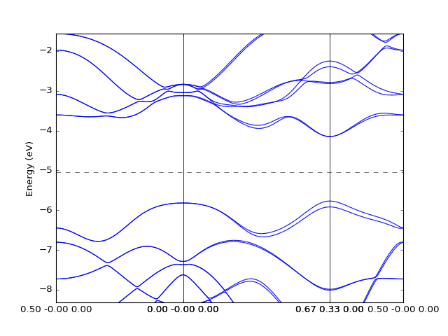
Example: OpenMX
In this case to retrieve the band structure we import parser
dfttools.parsers.openmx.bands explicitly.
from dfttools.parsers.openmx import bands
from dfttools import presentation

from matplotlib import pyplot

with open("plot.py.data",'r') as f:

    # Read bands data
    b = bands(f.read()).bands()

    # Plot bands
    presentation.matplotlib_bands(b,pyplot.gca())
    pyplot.show()
(Source code, png, hires.png, pdf)

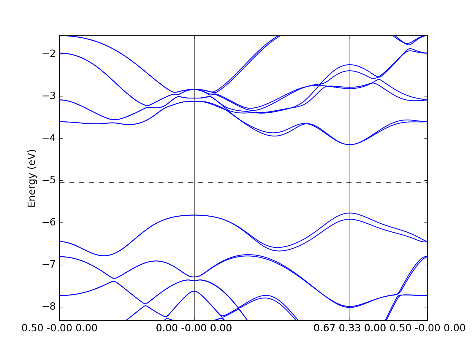
Example: Quantum Espresso
The Quantum Espresso files can be identified automatically via
dfttools.simple.parse routine.
from dfttools.simple import parse
from dfttools import presentation

from matplotlib import pyplot

with open("plot.py.data",'r') as f:

    # Read bands data
    bands = parse(f, "band-structure")

    # Plot bands
    presentation.matplotlib_bands(bands,pyplot.gca())
    pyplot.show()
(Source code, png, hires.png, pdf)

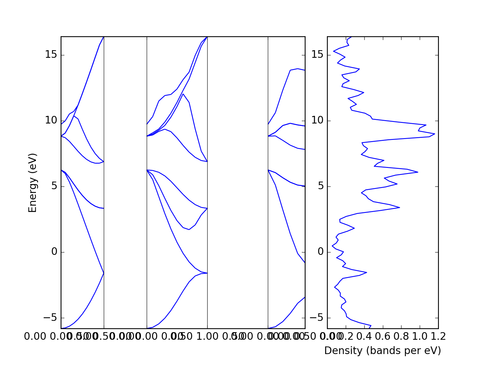
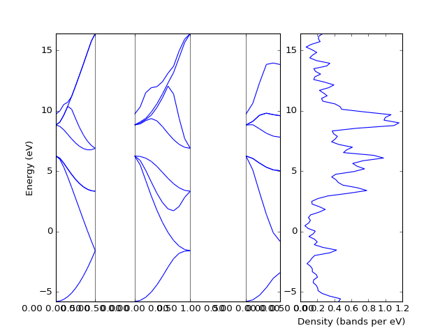
The density of states can be plotted directly from the band structure. However, one has to note that the density calculated from a k-point path is usually not the relevant one.
from dfttools.simple import parse
from dfttools import presentation

from matplotlib import pyplot

with open("plot.py.data",'r') as f:

    # Read bands data
    bands = parse(f, "band-structure")

    # Prepare axes
    ax_left  = pyplot.subplot2grid((1,3), (0, 0), colspan=2)
    ax_right = pyplot.subplot2grid((1,3), (0, 2))

    # Plot bands
    presentation.matplotlib_bands(bands,ax_left)
    presentation.matplotlib_bands_density(bands, ax_right, 100, orientation = 'portrait')
    ax_right.set_ylabel('')
    pyplot.show()
(Source code, png, hires.png, pdf)
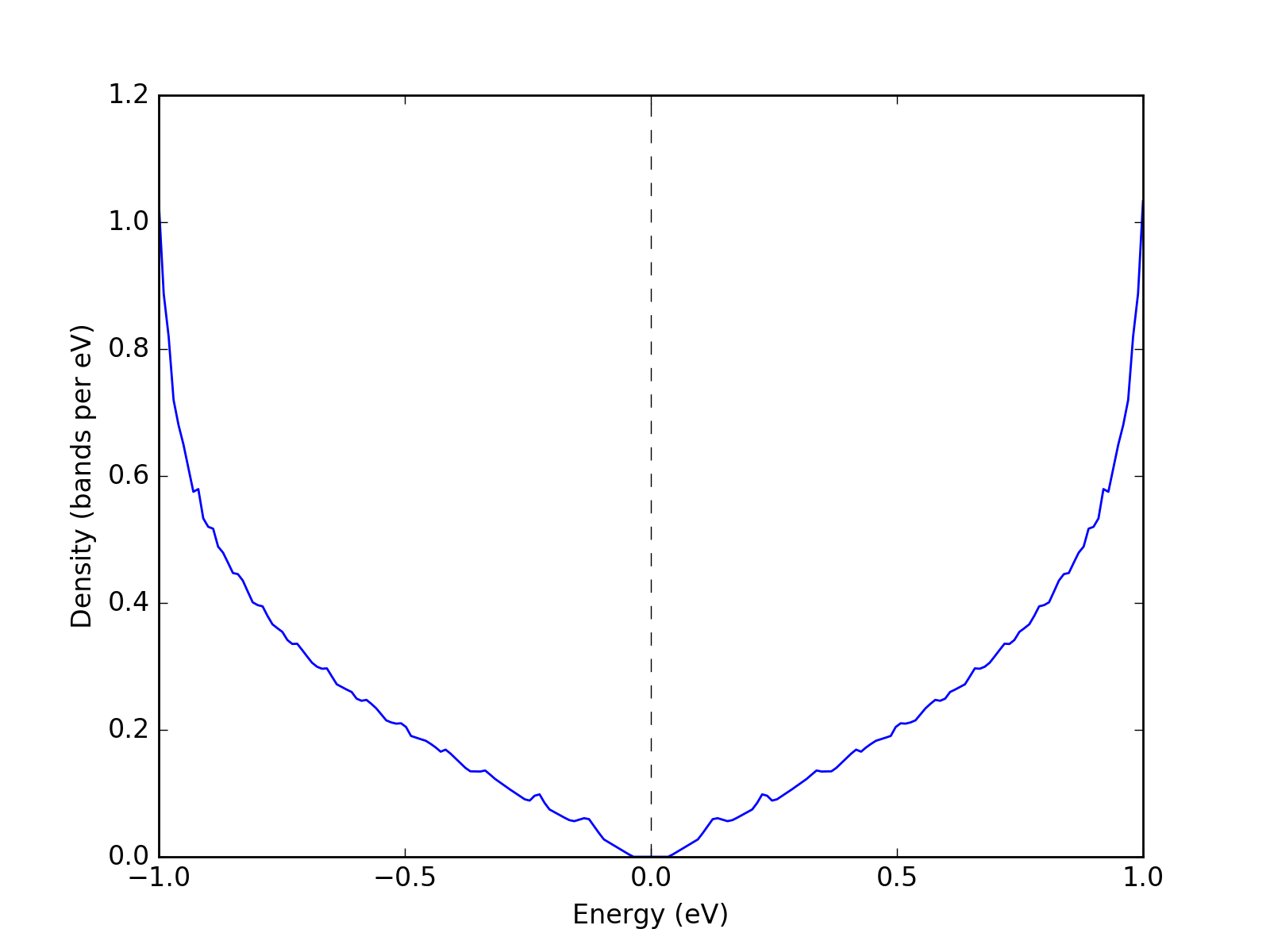
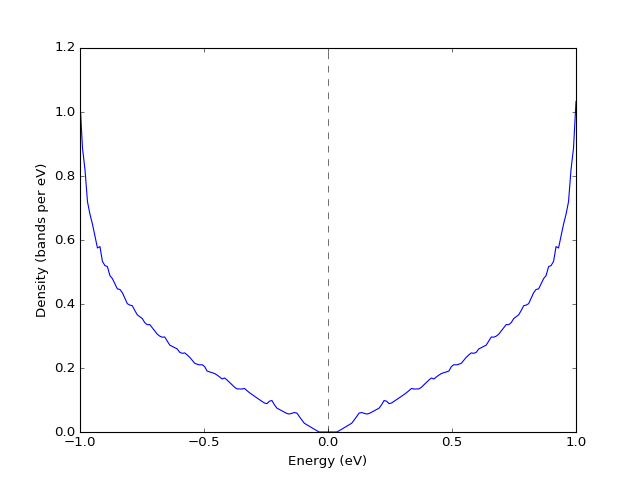
Example: Density of states
To plot an accurate density of states (DoS) a large enough grid is required. Following is an example of a density of states of graphene.
from dfttools.types import Basis, Grid
from dfttools import presentation

from matplotlib import pyplot
from numericalunits import eV
import numpy

# A reciprocal basis
basis = Basis((1,1,1,0,0,-0.5), kind = 'triclinic', meta = {"Fermi": 0})

# Grid shape
shape = (50,50,1)

# A dummy grid with correct grid coordinates and empty grid values
grid = Grid(
    basis,
    tuple(numpy.linspace(0,1,x, endpoint = False)+.5/x for x in shape),
    numpy.zeros(shape+(2,), dtype = numpy.float64),
)

# Calculate graphene band
k = grid.cartesian()*numpy.pi/3.**.5*2
e = (1+4*numpy.cos(k[...,1])**2 + 4*numpy.cos(k[...,1])*numpy.cos(k[...,0]*3.**.5))**.5*eV

# Set the band values
grid.values[...,0] = -e
grid.values[...,1] = e

presentation.matplotlib_bands_density(grid, pyplot.gca(), 200, energy_range = (-1, 1))
pyplot.show()
(Source code, png, hires.png, pdf)
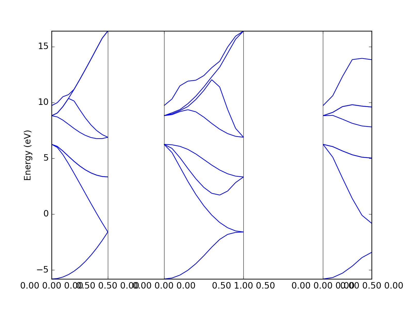
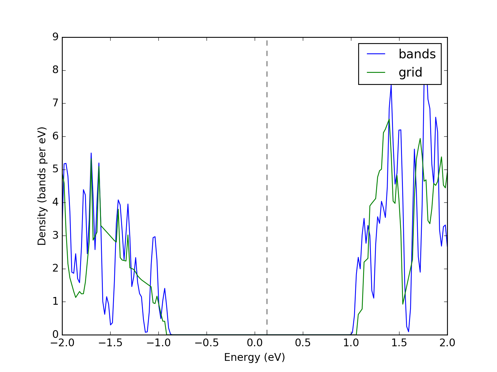
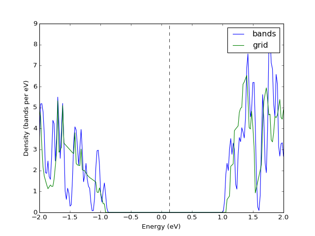
Example: K-point grids: density of states and interpolation
They key point of presenting the density of states from a file is
converting the band structure to grid via UnitCell.as_grid. This
only works if you indeed calculated band energies on a grid. Note
that while both Grid and UnitCell can be used for DoS, the
former one is considerably more accurate.
from dfttools.simple import parse
from dfttools import presentation

from matplotlib import pyplot

with open("plot.py.data",'r') as f:

    # Retrieve the last band structure from the file
    bands = parse(f, "band-structure")

    # Convert to a grid
    grid = bands.as_grid()

    # Plot both
    presentation.matplotlib_bands_density(bands, pyplot.gca(), 200, energy_range = (-2, 2), label = "bands")
    presentation.matplotlib_bands_density(grid,  pyplot.gca(), 200, energy_range = (-2, 2), label = "grid")
    pyplot.legend()
    pyplot.show()
(Source code, png, hires.png, pdf)
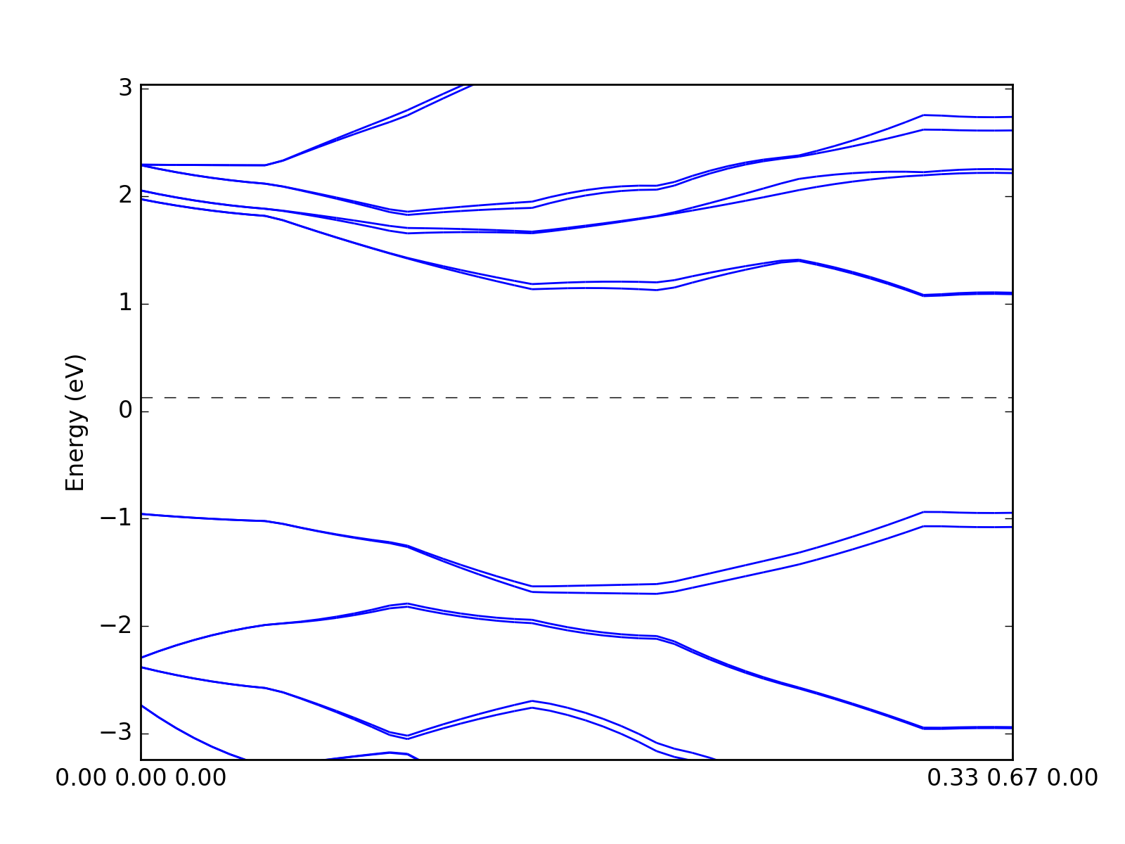
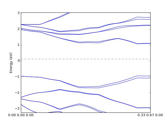
One can also plot the bands by interpolating data on the grid. The quality of the figure depends on the grid size and interpolation methods.
from dfttools.simple import parse
from dfttools import presentation

import numpy
from matplotlib import pyplot

with open("plot.py.data",'r') as f:

    # Retrieve the last band structure from the file
    bands = parse(f, "band-structure")

    # Convert to a grid
    grid = bands.as_grid()

    # Interpolate
    kp_path = numpy.linspace(0,1)[:,numpy.newaxis] * ((1./3,2./3,0),)
    bands = grid.interpolate_to_cell(kp_path)

    # Plot
    presentation.matplotlib_bands(bands, pyplot.gca())
    pyplot.show()
(Source code, png, hires.png, pdf)
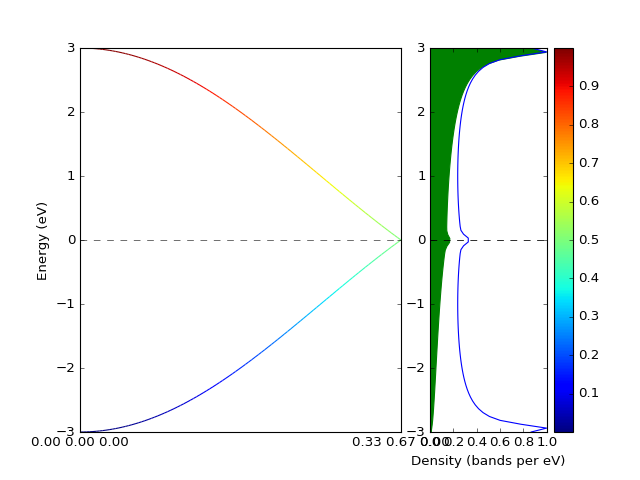
Example: Band structure with weights
The band structure with weights is plotted using weights keyword
argument. The weights array is just numbers assigned to each k-point and
each band.
from dfttools.types import Basis, UnitCell
from dfttools import presentation

from matplotlib import pyplot
from numericalunits import eV
import numpy

# A reciprocal basis
basis = Basis((1,1,1,0,0,-0.5), kind = 'triclinic', meta = {"Fermi": 0})

# G-K path
kp = numpy.linspace(0,1,100)[:,numpy.newaxis] * numpy.array(((1./3,2./3,0),))

# A dummy grid UnitCell with correct kp-path
bands = UnitCell(
    basis,
    kp,
    numpy.zeros((100,2), dtype = numpy.float64),
)

# Calculate graphene band
k = bands.cartesian()*numpy.pi/3.**.5*2
e = (1+4*numpy.cos(k[...,1])**2 + 4*numpy.cos(k[...,1])*numpy.cos(k[...,0]*3.**.5))**.5*eV

# Set the band values
bands.values[...,0] = -e
bands.values[...,1] = e

# Assign some weights
weights = bands.values.copy()
weights -= weights.min()
weights /= weights.max()

# Prepare axes
ax_left  = pyplot.subplot2grid((1,3), (0, 0), colspan=2)
ax_right = pyplot.subplot2grid((1,3), (0, 2))

# Plot bands
p = presentation.matplotlib_bands(bands,ax_left,weights = weights)
presentation.matplotlib_bands_density(bands, ax_right, 100, orientation = 'portrait')
presentation.matplotlib_bands_density(bands, ax_right, 100, orientation = 'portrait', weights = weights, use_fill = True, color = "#AAAAFF")

ax_right.set_ylabel('')
pyplot.colorbar(p)
pyplot.show()
(Source code, png, hires.png, pdf)
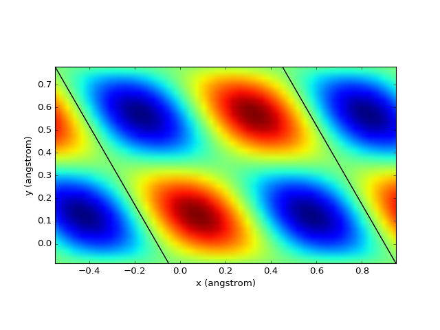
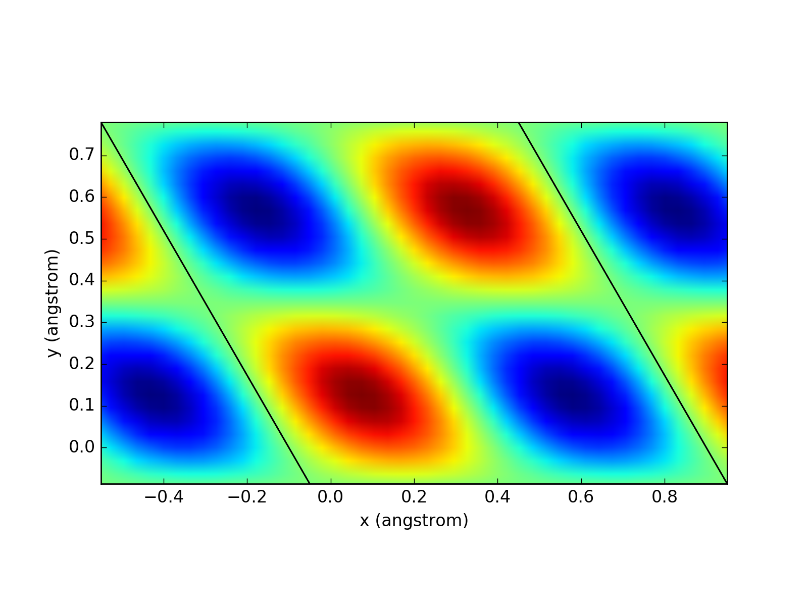
Data on the grid
Plotting of data (charge, potential, density, etc.) on a 3D grid is very straightforward.
from dfttools.types import Basis, Grid
from dfttools import presentation

from numericalunits import angstrom
from matplotlib import pyplot
import numpy

grid = Grid(
    Basis((1*angstrom,1*angstrom,1*angstrom,0,0,-0.5), kind = 'triclinic'),
    (
        numpy.linspace(0,1,30,endpoint = False),
        numpy.linspace(0,1,30,endpoint = False),
        numpy.linspace(0,1,30,endpoint = False),
    ),
    numpy.zeros((30,30,30)),
)
grid.values = numpy.prod(numpy.sin(grid.explicit_coordinates()*2*numpy.pi), axis = -1)

presentation.matplotlib_scalar(grid, pyplot.gca(), (0.1,0.1,0.1), 'z', show_cell = True)
pyplot.show()
(Source code, png, hires.png, pdf)