Introduction to DFT Tools

A number of codes implementing DFT and it’s flavors is available in the web, see Wikipedia for example. The developers of these codes are usually scientists who never aimed to develop a user-friendly application mainly because they are not get paid for that. Thus, to be able to use such codes one has to master several tools, among which is data post-processing and presentation.

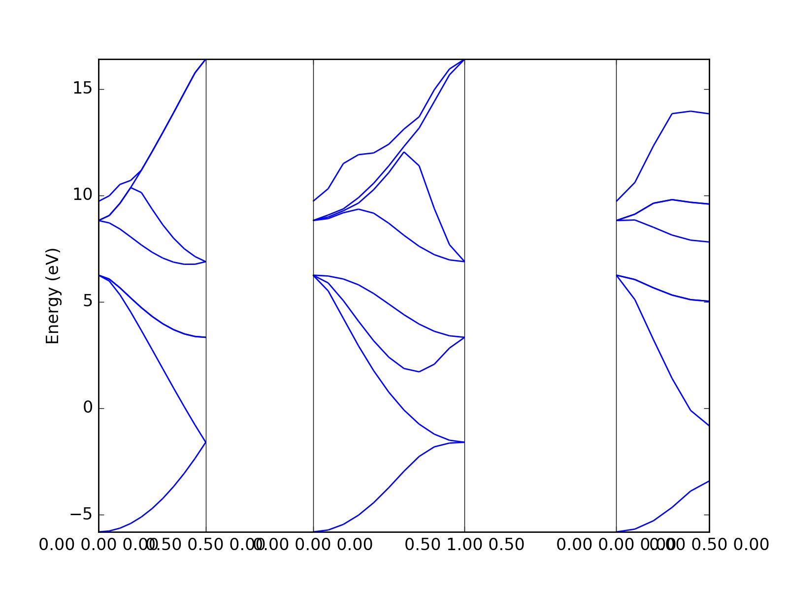
An average DFT code produces a set of text and binary data during the run. Typically, the data cannot be plotted directly and one needs a program to collect this data and present it. Here is an example of a Quantum Espresso band structure:

          k = 0.0000 0.0000 0.0000     band energies (ev):

    -5.8099   6.2549   6.2549   6.2549   8.8221   8.8221   8.8221   9.7232

          k = 0.0000 0.0000 0.1000     band energies (ev):

    -5.7668   5.9810   6.0722   6.0722   8.7104   9.0571   9.0571   9.9838

          k = 0.0000 0.0000 0.2000     band energies (ev):

    -5.6337   5.3339   5.6601   5.6601   8.4238   9.6301   9.6301  10.5192

With DFT Tools it can be plotted as easy as is following script:

from dfttools.simple import parse
from dfttools import presentation

from matplotlib import pyplot

with open("plot.py.data",'r') as f:

    # Read bands data
    bands = parse(f, "band-structure")

    # Plot bands
    presentation.matplotlib_bands(bands,pyplot.gca())
    pyplot.show()

(Source code, png, hires.png, pdf)

Not only the band structure can be plotted, but atomic structure, data on the grid, etc., see examples.